Did Your LLM Actually Read That File?

Your coding agent just read twelve files, ran three shell commands, and confidently told you the server config is wrong. Or you pasted those files into a chat and asked the same question. Either way, the LLM answered from a long context. Which of those twelve files did its answer actually rest on? Did the lsof output matter? Did it ignore the config file it so dutifully opened?

You can’t just ask it; models make up plausible justifications. Attention maps feel like the answer but are famously unreliable as explanations. There is a better way, and it needs nothing but forward passes and a linear regression: ablation attribution, published as ContextCite by Cohen-Wang et al. (NeurIPS 2024).

Keep the model’s answer fixed, remove one source at a time, and measure how much less likely that same answer becomes. A source whose removal makes the answer collapse is a source the answer rested on. This post builds the method from scratch, following the confusions I had when learning it. It ends with what the method cannot tell you, and with a test of whether it finds the right source when we know the answer.

Two corrections to the first instinct

If you come from classical ML, “attribute the output to the input” sounds like a saliency map: an importance score for every input token. That instinct is half right (this method is a cousin of SHAP), but it needs two corrections.

Attribute to sources, not tokens. Nobody cares whether input token 4,812 mattered. You care whether the config file mattered. So the context is cut into a handful of sources: one file read, one tool result, one instruction block. A real context has maybe 5 to 50 sources, not 30,000 tokens. Call that number $d$; keeping it small is what makes everything affordable.

Never attribute the generation; attribute the score of a fixed answer. An LLM’s output is sampled: run it twice and you may get different answers. “How much did source B influence the output” is ill-defined when the output itself is a dice roll. So the model generates its answer exactly once, and from then on we never generate again. We use the model’s other mode:

• Generate: “here’s a prompt, produce an answer.” Sampled, slow, one token at a time.
• Grade: “here’s a prompt and a finished answer; how probable would you have found these exact tokens?” Deterministic, no sampling at all.

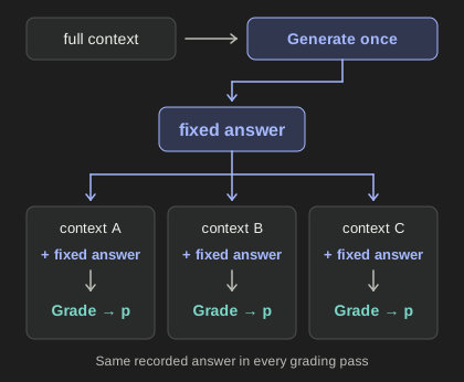
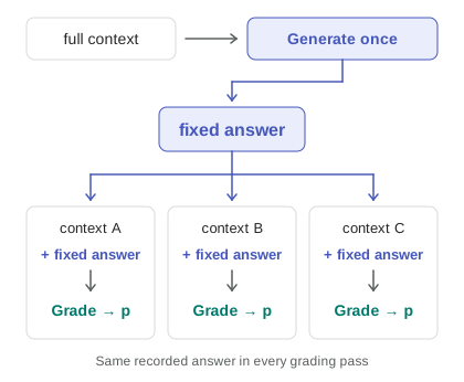
Grading gives one number for any context: the probability $p$ the model assigns to the recorded answer (for a multi-token answer, the product over its tokens). ContextCite works with its log-odds:

$\text{score}=\log \frac{p}{1-p}$

Why log-odds and not $p$ itself? Probabilities are squeezed into $[0,1]$, so near the edges big changes look tiny: going from 90% to 95% barely moves $p$, but it doubles the odds (9 to 1 becomes 19 to 1). Log-odds stretch the scale so that such changes count, which is what a linear regression needs.

Why grading is cheap: one pass instead of many

Generation is sequential: one forward pass per new token. Grading has no unknowns; the full sequence (context plus fixed answer) goes through in one parallel forward pass, and the causal attention mask makes sure each position is scored using only the tokens before it. It is exactly how models are trained: a training step scores a known text in one pass. Grading is a training step without the weight update. A 500-token answer costs one pass over 500 tokens, not 500 sequential steps.

We have turned a sampling machine into a deterministic function: give it any modified context plus the fixed answer, get back one score. Now we can experiment on that function.

An example, step by step

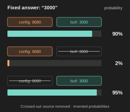
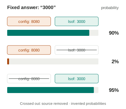
The context holds a question (“What port is the server on? Reply with just the number.”), a config file that says port = 8080, and an lsof tool result that says the server listens on port 3000. The model answered once: 3000. (The probabilities below are invented for illustration, and I treat “3000” as a single token.)

• Both sources kept. The model gives “3000” a probability of 90%.
• The lsof result removed. “Ablating” is physically dumb: delete the source’s tokens and grade the same answer again. Now the model would much rather say “8080” (93%), but we never let it say anything. We only read the probability of the recorded “3000”: a miserable 2%. This exact answer became 45 times less likely.
• The config file removed. “3000” goes up, to 95%. The config file was a distractor, mildly pushing against the answer.

From ablations to attributions

Collect the experiments into a table, including one with both sources removed:

config file	lsof result	$p$(“3000”)	log-odds
kept	kept	0.90	+2.20
kept	removed	0.02	−3.89
removed	kept	0.95	+2.94
removed	removed	0.04	−3.14

Now fit a linear regression: $\text{score}\approx \text{base}+w_{\text{config}}\cdot \text{config}+w_{\text{lsof}}\cdot \text{lsof}$, where each source is 1 when kept and 0 when removed. (The invented values were chosen so this fit is exact.)

The weights are signed, and a negative weight is a real finding: a source that pushed against the answer. They also have a clean reading. Because they add in log-odds, each kept source multiplies the odds of the answer by $e^w$: the lsof result by about 440, the config file by about one half.

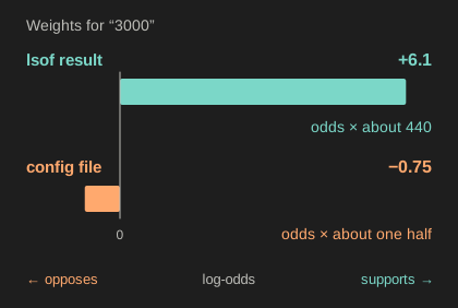
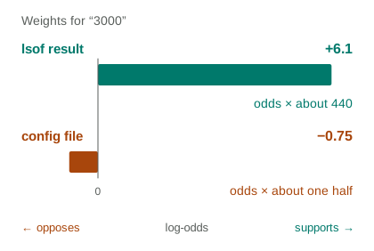
A single ablation only tells you about one combination of sources. The regression over many combinations is what separates each source’s individual share. The linear model is not the idea; it is the tool that turns mixed evidence into one number per source.

”But that’s $2^d$ forward passes!”

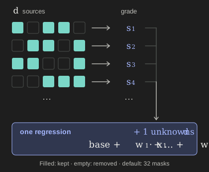
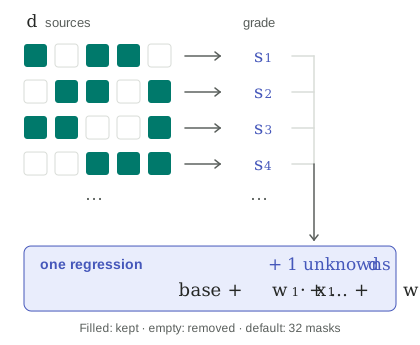
With $d$ sources there are $2^d$ possible subsets to remove. For 30 sources, a billion. Luckily you don’t need all of them. You need $d+1$ regression coefficients, and fitting $d+1$ unknowns needs on the order of $d$ measurements, not $2^d$, for the same reason fitting a plane doesn’t require measuring every point in space.

So: sample a few dozen random keep-or-remove masks (each source kept with probability ½), grade each one, fit the regression. The paper’s default is 32 masks. It also fits with Lasso, betting that only a handful of sources really matter, which lets it get away with even fewer. On a single consumer GPU with a 7B model, this takes a few minutes per answer.

Checking the fit, per answer

At this point you should be suspicious. A linear stand-in for a transformer, fitted on 32 samples?

You don’t have to take it on faith; you can check it. Keep some sampled masks out of the fit, ask the fitted line to predict their scores, and compare with what the model actually gave, using a rank correlation. The paper calls this the linear datamodeling score (LDS) and uses it to evaluate the method. You can run the same check on any single answer: a high score means the linear story predicts what removing things does for this answer; a low score means the weights are not worth quoting here.

Where linearity breaks: redundant sources

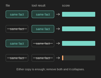
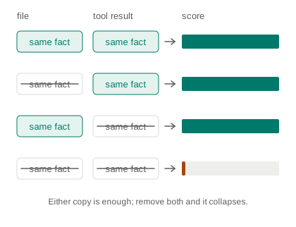
Suppose two sources carry the same fact (a file read twice, or a tool result quoting the file). Remove either alone: nothing happens. Remove both: the score collapses. That is an OR, and a linear model cannot represent it at any sample size; more samples reduce noise, not the wrong shape of the model. The authors document this case. The danger is that the check above can look fine while the two copies quietly split or hide their credit. If your context repeats itself, add targeted experiments that remove both copies together.

What it can never tell you

We measured that the probability of “3000” collapses without the lsof result. Does that tell you what the model would have done without it?

No, and it can’t. The method only grades the answer that actually happened. It knows that answer becomes unlikely without the source; it cannot know what would have replaced it. Maybe a paraphrase (“the server is on port 3000”), in which case the behavior didn’t depend on the source at all, only the exact wording did. Finding out requires generating again under the ablated context, which is a different and more expensive experiment.

So read the weights as: this source supported the answer as written. That is reliance, not understanding. A model can lean on exactly the right file and still misread it. The next posts look inside the model for that: how attention carries a source into the answer, which heads do it, and whether they can tell a right reading from a wrong one.

Does it find the right source?

A method like this is only worth using if it finds the right source when we know what the right source is. So I tested it. I wrote 12 small contexts, each with 10 sources: nine realistic snippets from real open-source projects, and one that plants an invented fact the question needs (invented, so the model cannot know it from training). Qwen2.5-Coder-7B answered each question 5 times, and ContextCite ranked the sources for every answer. One context failed a check set in advance and was dropped, leaving 11.

The planted source came out first in 55 of 55 runs. Picking at random would get that right 10% of the time. A keyword search (BM25) that matches the question’s words against the sources ranked the planted source first for only 4 of the 11 contexts, so the method is not just matching words. And the same method on a copy of the model with random weights ranked it first for only 2 of 11, so the signal comes from what the trained model actually does with the text.

Within its scope, that is a remarkable deal: a per-answer, testable attribution for the price of a few dozen forward passes and a Lasso fit, with no access to the model’s insides beyond probabilities.

---

Revised on 2026-09-26: retitled from “Did Your Agent Actually Read That File?”, with new figures, a few corrections and a validation test.

References.

• Cohen-Wang, Shah, Georgiev, Madry, “ContextCite: Attributing Model Generation to Context,” NeurIPS 2024, arXiv 2409.00729; reference implementation MadryLab/context-cite. Their Appendix C.4 lists four documented failure modes and is worth reading.
• Robertson and Zaragoza, “The Probabilistic Relevance Framework: BM25 and Beyond,” Foundations and Trends in Information Retrieval, 2009.