How Does an LLM Read Its Context?

The context says: “Logs rotate daily. The timeout is half a minute. Retries use backoff.” The question is “How many seconds is the timeout?” Suppose the LLM answers “30”, although “30” appears nowhere in the text. How does information from “half a minute” reach that answer? We will follow it through attention, from the tokens the model reads to the vectors its heads write.

A vector at every position

First, the model splits the text into tokens: pieces that can be words, parts of words, or punctuation. It looks up an embedding for each token, a learned list of numbers called a vector. A position starts with that embedding and carries an evolving vector through a stack of layers. The vector can come to represent much more than the token that started it.

In Qwen3-0.6B, each of these vectors has 1,024 numbers and passes through 28 layers. Qwen3-8B uses 4,096 numbers and 36 layers. These are the dimensions of the vectors carried between layers, not the sizes of individual heads. (0.6B configuration, 8B configuration)

Below, each little stack stands for a whole vector. Let us follow any column upward: the token stays at its position while its representation changes. I show selected text pieces and an abbreviated layer stack, not an exact tokenizer output.

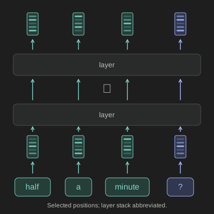
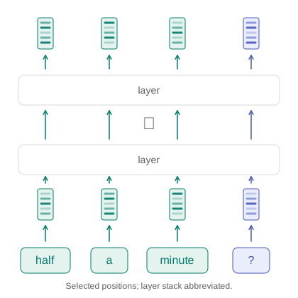
For this invented example, I treat “30” as one token; a real tokenizer may split it. We will follow the position whose vector predicts “30”. We call this the answer position. It is the last position already supplied to the model when that token is predicted, not a slot that already contains “30”.

Attention gathers information

A vector at the answer position needs information from elsewhere. Attention lets it gather a weighted mixture of information from the available positions. In a causal language model, it can use earlier positions and itself, never future positions. “Looking backward” means backward through the text, not down through earlier layers.

An attention head makes a query from the receiving position and a key and value from each source position. Think of the query as a search request, the key as something to match against, and the value as the information available to carry back. They are all vectors, made by learned matrix multiplications:

$$q_t=W_Q{x}_t,k_j=W_K{x}_j,v_j=W_V{x}_j.$$

Here $t$ is the receiving position, $j$ a source position, and $x$ the vector supplied to attention. The matrices are learned transformations, not text searches. A dot product multiplies corresponding entries and adds the results. The head uses it to score how well the query and each key line up.

It scales those scores by the square root of the head size $d_h$, then applies softmax: exponentiate each score and divide by the total. This makes nonnegative attention weights ${\alpha }_j$ that sum to $1$ over the permitted positions:

$$s_j=\frac{q_t\cdot k_j}{\sqrt{d_h}},{\alpha }_j=\frac{\exp (s_j)}{{\sum }_{i\le t}\exp (s_i)},j\le t.$$

The value takes a separate route. An output matrix $W_O$ maps it back to the width of the vector between layers. The head scales each resulting vector by its attention weight and adds them:

$$c_t=\sum _{j\le t}{\alpha }_j{W}_O{v}_j.$$

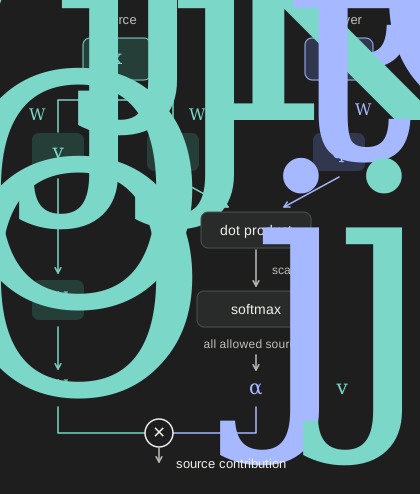
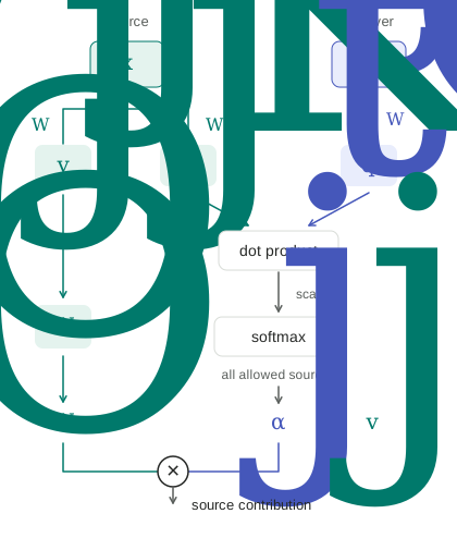
The diagram follows one source through those routes. On the right, its key meets the receiving query to determine a weight. On the left, its value becomes a vector to write. They meet at multiplication; summing these contributions over sources gives the head’s output.

Normalization and position encoding

These equations leave out normalization and position encoding to expose the routing. In Qwen3, attention reads normalized vectors; queries and keys also undergo normalization and positional rotation before scoring. Those steps change the scores, but preserve the distinction between choosing a source and transforming its value. (Qwen3 implementation)

Many heads, many places to look

A layer runs many heads side by side. In ordinary multi-head attention, each has its own $W_Q$, $W_K$, $W_V$, and $W_O$, so heads can learn different matching rules and different transformations. Qwen3 shares key and value matrices among groups of heads, while each query head still has its own query map and output slice. Sharing some machinery does not force the heads to look at the same places.

Qwen3-0.6B has 16 query heads per layer, with 128 numbers in each head’s query, key, or value vector. Qwen3-8B has 32 query heads per layer. The output projection brings each head’s result back to the model’s vector width so their contributions can be added. (0.6B configuration, 8B configuration)

Let us look at two illustrative heads in the same layer at the answer position. Attention is over tokens. I group them into the start of context, S1 (“Logs rotate daily”), S2 (the timeout fact), S3 (“Retries use backoff”), and Q (the question) only to summarize it: a sentence’s attention is the sum over its tokens. Each line below carries that sum for its part. Thicker means more attention, with the same scale for both heads.

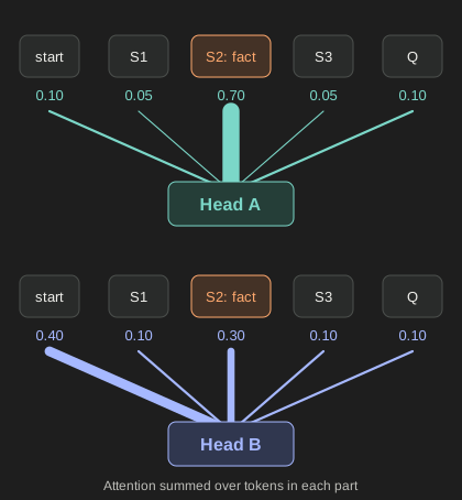
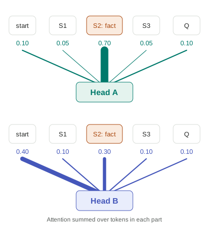
Head A gives the fact $0.70$ of its attention. Head B gives it $0.30$, and gives the start $0.40$. Heavy attention to initial positions is a common habit called an attention sink; a thick line there need not mean important factual content. These weights are illustrative, not measurements from Qwen. (Attention sinks)

If looking were the whole job, A would seem the better candidate. We still need to see what arrived.

Each head adds to a shared vector

The vector moving up the layers is called the residual stream. A head does not replace it. Each head adds its output to the receiving position’s existing vector. Then the layer’s MLP, a neural network that transforms each position separately, adds another update. Later layers read the result and repeat the process.

The next picture follows just the answer position through a layer. The main vertical path continues past the side branches. Heads and the MLP read from it and return additions at the plus signs.

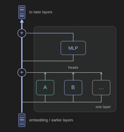
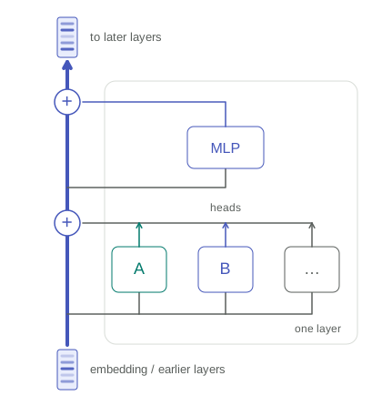
If we unroll all those additions, the final residual vector $r_t$ is the original embedding $e_t$ plus every head contribution $c_{\ell ,h,t}$ and every MLP contribution $m_{\ell ,t}$ at that position:

$$r_t=e_t+\sum _{\ell }\sum _h{c}_{\ell ,h,t}+\sum _{\ell }{m}_{\ell ,t}.$$

This is why we can isolate what a particular head added in a particular forward pass. The sum is exact, but its terms are not independent computations: later heads and MLPs depend on earlier additions. Removing a head and running the model again can change those later terms too.

One head reads; the same head writes

There are two distinct jobs inside a head. Read, controlled by query and key, chooses the weights. Write, controlled by value and output, determines what gets added from each source. Their parameters are separate: knowing the attention weights does not tell us the direction of the written vector. A head can look hard at the correct sentence and write nothing useful toward the answer.

For this example, we can compress the write into coordinates called “toward 30” and “other”. Before attention weighting, let A’s write from the fact be $(0.1,1.0)$ and B’s be $(3.0,0.2)$. A writes mostly in the other direction. B writes strongly toward “30”. These are invented vectors for explaining the mechanism.

What a write from a sentence means

Because the fact spans several tokens, “write from the fact” here means the attention-weighted average of their $W_O{v}_j$ vectors, before multiplying by the fact’s total attention. This keeps the span illustration consistent with the token-level sum.

The missing piece is what “toward 30” means inside a model.

Measure the shadow toward the answer

At the top, the model scores every token in its vocabulary. Each token $y$ has a row $u_y$ in the unembedding matrix. Its score, called a logit, is a dot product with the final vector presented to that matrix:

$$\mathrm{logit}(y)=u_y\cdot z_t.$$

Here $z_t$ is the final residual vector after the model’s final normalization. Picture $u_{30}$ as an arrow pointing toward a higher score for “30”. A contribution pointing along it helps that score; a contribution pointing across it can be large yet give little help. Its dot product is like a signed shadow on the answer direction, scaled by the length of the unembedding vector.

For the picture, I make $u_{30}$ a unit arrow along the horizontal axis. Attention shrinks each write before we measure its shadow. Both panels use the same scale: the faint arrow is the write before weighting, the solid arrow is the weighted contribution, and the thick horizontal segment is its shadow.

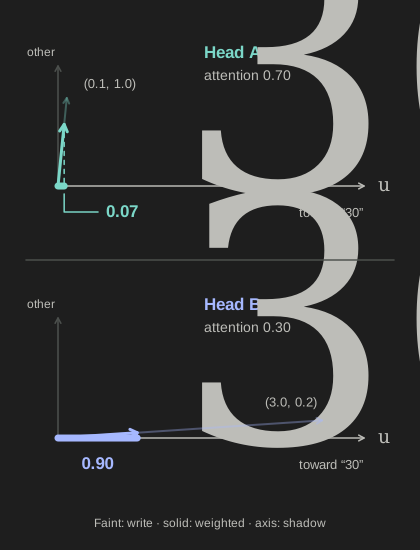
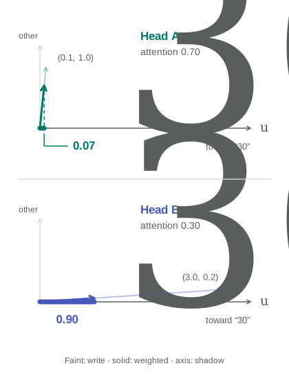
Head A’s push from the fact is $0.70\times 0.1=0.07$. Head B’s is $0.30\times 3.0=0.90$. More attention, less push. Nothing requires the source text to contain “30”: the value and output maps transform a contextual representation, rather than copying its token label. The example does not assign the entire conversion from minutes to seconds to one head.

A projection is not a causal effect

One precision matters: Qwen’s final normalization sits between the additive residual stream and the logits. The shadow is therefore a direct-path view of a head’s contribution, not an exact change in the emitted logit or answer probability. It also leaves out what later heads and MLPs do with that contribution.

Attention tells us where a head reads. Its value and output maps tell us what it writes. In this example, the head that pays less attention to the fact supplies the larger push toward the answer. That gives us a way to ask a more specific question about a real LLM: Which Heads Read Your Context? follows this machinery to find the heads that carry a fact into the answer.

References.

• Elhage et al., “A Mathematical Framework for Transformer Circuits,” Anthropic, 2021.
• Xiao, Tian, Chen, Han, Lewis, “Efficient Streaming Language Models with Attention Sinks,” arXiv 2309.17453.
• Qwen Team, “Qwen3 model configurations,” Qwen3-0.6B and Qwen3-8B.
• Hugging Face contributors, “Qwen3 implementation,” Transformers source.