Note
This tutorial is available as a Jupyter notebook. Download notebook
Tutorial 03: Binary Classification#
🟢 Beginner — No prior boosting experience needed
Learn how to train a binary classifier with boosters and evaluate it using ROC curves and AUC.
What you’ll learn#
Train a binary classifier
Get probability predictions
Plot ROC curves and calculate AUC
Choose classification thresholds
[1]:
import numpy as np
import matplotlib.pyplot as plt
from sklearn.datasets import make_classification
from sklearn.model_selection import train_test_split
from sklearn.metrics import roc_curve, auc, precision_recall_curve, classification_report

from boosters.sklearn import GBDTClassifier
Generate Data#
Create a binary classification dataset:
[2]:
# Generate binary classification data
X, y = make_classification(
    n_samples=2000,
    n_features=20,
    n_informative=10,
    n_redundant=5,
    n_classes=2,
    weights=[0.7, 0.3],  # Slight imbalance
    random_state=42
)

X_train, X_test, y_train, y_test = train_test_split(X, y, test_size=0.2, random_state=42)

print(f"Training samples: {len(X_train)}")
print(f"Class distribution: {np.bincount(y_train)}")
Training samples: 1600
Class distribution: [1121  479]
Train the Classifier#
[3]:
# Train classifier
clf = GBDTClassifier(
    n_estimators=100,
    max_depth=6,
    learning_rate=0.1,
)
clf.fit(X_train, y_train)

print(f"Accuracy: {clf.score(X_test, y_test):.4f}")
Accuracy: 0.9300
Probability Predictions#
[4]:
# Get probability predictions
y_proba = clf.predict_proba(X_test)
y_score = y_proba[:, 1]  # Probability of positive class

print(f"Probability shape: {y_proba.shape}")
print(f"Sample probabilities: {y_score[:5]}")
Probability shape: (400, 2)
Sample probabilities: [0.00366234 0.00452526 0.6404448  0.05477158 0.8995941 ]
ROC Curve and AUC#
[5]:
# Calculate ROC curve
fpr, tpr, thresholds = roc_curve(y_test, y_score)
roc_auc = auc(fpr, tpr)

# Plot
plt.figure(figsize=(8, 6))
plt.plot(fpr, tpr, color='blue', lw=2, label=f'ROC curve (AUC = {roc_auc:.3f})')
plt.plot([0, 1], [0, 1], color='gray', lw=1, linestyle='--', label='Random')
plt.xlabel('False Positive Rate')
plt.ylabel('True Positive Rate')
plt.title('Receiver Operating Characteristic (ROC)')
plt.legend(loc='lower right')
plt.grid(True, alpha=0.3)
plt.show()

print(f"AUC: {roc_auc:.4f}")
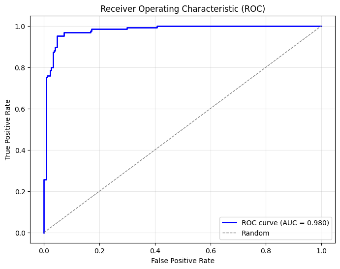
AUC: 0.9799
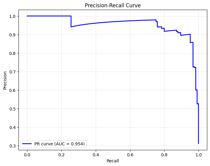
Precision-Recall Curve#
[6]:
# Calculate precision-recall curve
precision, recall, thresholds_pr = precision_recall_curve(y_test, y_score)
pr_auc = auc(recall, precision)

# Plot
plt.figure(figsize=(8, 6))
plt.plot(recall, precision, color='blue', lw=2, label=f'PR curve (AUC = {pr_auc:.3f})')
plt.xlabel('Recall')
plt.ylabel('Precision')
plt.title('Precision-Recall Curve')
plt.legend(loc='lower left')
plt.grid(True, alpha=0.3)
plt.show()
Classification Report#
[7]:
# Get class predictions
y_pred = clf.predict(X_test)

# Print classification report
print(classification_report(y_test, y_pred, target_names=['Negative', 'Positive']))
              precision    recall  f1-score   support

    Negative       0.93      0.97      0.95       275
    Positive       0.92      0.85      0.88       125

    accuracy                           0.93       400
   macro avg       0.93      0.91      0.92       400
weighted avg       0.93      0.93      0.93       400
Summary#
In this tutorial, you learned how to:
✅ Train a binary classifier
✅ Get probability predictions with
predict_proba✅ Plot ROC curves and calculate AUC
✅ Analyze precision-recall trade-offs
Next Steps#
Tutorial 04: Multiclass Classification — Handle multiple classes
Tutorial 05: Early Stopping — Prevent overfitting