Note
This tutorial is available as a Jupyter notebook. Download notebook
Tutorial 05: Early Stopping#
🟡 Intermediate — Familiarity with ML concepts helpful
Learn how to use early stopping to prevent overfitting and find the optimal number of trees.
What you’ll learn#
Understand the overfitting problem
Use validation-based early stopping
Visualize training curves
Choose early stopping parameters
[1]:
import numpy as np
import matplotlib.pyplot as plt
from sklearn.datasets import make_regression
from sklearn.model_selection import train_test_split
from sklearn.metrics import mean_squared_error

from boosters.sklearn import GBDTRegressor
The Overfitting Problem#
Without early stopping, adding more trees can lead to overfitting:
[2]:
# Generate data with some noise
X, y = make_regression(n_samples=500, n_features=10, noise=10.0, random_state=42)

# Split data
X_train, X_temp, y_train, y_temp = train_test_split(X, y, test_size=0.4, random_state=42)
X_val, X_test, y_val, y_test = train_test_split(X_temp, y_temp, test_size=0.5, random_state=42)

print(f"Train: {len(X_train)}, Validation: {len(X_val)}, Test: {len(X_test)}")
Train: 300, Validation: 100, Test: 100
Training Without Early Stopping#
[3]:
# Train with many trees
model_no_es = GBDTRegressor(
    n_estimators=500,
    max_depth=6,
    learning_rate=0.1,
)
model_no_es.fit(X_train, y_train)

# Evaluate
train_rmse = np.sqrt(mean_squared_error(y_train, model_no_es.predict(X_train)))
val_rmse = np.sqrt(mean_squared_error(y_val, model_no_es.predict(X_val)))
test_rmse = np.sqrt(mean_squared_error(y_test, model_no_es.predict(X_test)))

print(f"Without early stopping:")
print(f"  Train RMSE: {train_rmse:.4f}")
print(f"  Val RMSE:   {val_rmse:.4f}")
print(f"  Test RMSE:  {test_rmse:.4f}")
Without early stopping:
  Train RMSE: 0.0747
  Val RMSE:   62.7528
  Test RMSE:  64.3740
Early Stopping in Action#
Use early stopping to find the optimal number of iterations.
Note: Early stopping support depends on the API version. Here we demonstrate the concept by training multiple models:
[4]:
# Track errors across iterations
n_estimators_list = [10, 25, 50, 100, 150, 200, 300, 400, 500]
train_errors = []
val_errors = []

for n_est in n_estimators_list:
    model = GBDTRegressor(
        n_estimators=n_est,
        max_depth=6,
        learning_rate=0.1,
    )
    model.fit(X_train, y_train)

    train_rmse = np.sqrt(mean_squared_error(y_train, model.predict(X_train)))
    val_rmse = np.sqrt(mean_squared_error(y_val, model.predict(X_val)))

    train_errors.append(train_rmse)
    val_errors.append(val_rmse)

# Find best iteration
best_idx = np.argmin(val_errors)
best_n_estimators = n_estimators_list[best_idx]
print(f"Best n_estimators: {best_n_estimators} (val RMSE: {val_errors[best_idx]:.4f})")
Best n_estimators: 500 (val RMSE: 62.7528)
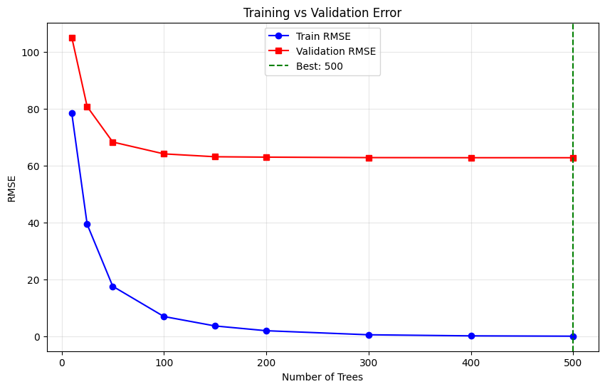
Visualize Training Curves#
[5]:
plt.figure(figsize=(10, 6))
plt.plot(n_estimators_list, train_errors, 'b-', label='Train RMSE', marker='o')
plt.plot(n_estimators_list, val_errors, 'r-', label='Validation RMSE', marker='s')
plt.axvline(x=best_n_estimators, color='g', linestyle='--', label=f'Best: {best_n_estimators}')
plt.xlabel('Number of Trees')
plt.ylabel('RMSE')
plt.title('Training vs Validation Error')
plt.legend()
plt.grid(True, alpha=0.3)
plt.show()
Train with Optimal Number of Trees#
[6]:
# Train with optimal n_estimators
model_optimal = GBDTRegressor(
    n_estimators=best_n_estimators,
    max_depth=6,
    learning_rate=0.1,
)
model_optimal.fit(X_train, y_train)

# Evaluate on test
test_rmse_optimal = np.sqrt(mean_squared_error(y_test, model_optimal.predict(X_test)))

print(f"With optimal trees ({best_n_estimators}):")
print(f"  Test RMSE: {test_rmse_optimal:.4f}")
print(f"\nImprovement over 500 trees: {test_rmse - test_rmse_optimal:.4f}")
With optimal trees (500):
  Test RMSE: 64.3740

Improvement over 500 trees: 0.0000
Summary#
In this tutorial, you learned:
✅ More trees doesn’t always mean better performance
✅ How to find optimal number of iterations using validation data
✅ How to visualize train/validation curves
✅ The importance of a held-out validation set
Next Steps#
Tutorial 06: GBLinear & Sparse Data — Linear boosting
Tutorial 07: Hyperparameter Tuning — Systematic optimization