Note
This tutorial is available as a Jupyter notebook. Download notebook
Tutorial 04: Multiclass Classification#
🟡 Intermediate — Familiarity with ML concepts helpful
Learn how to train a multiclass classifier using the softmax objective.
What you’ll learn#
Train a multiclass classifier
Interpret multiclass probabilities
Visualize confusion matrices
Handle class imbalance
[1]:
import numpy as np
import matplotlib.pyplot as plt
from sklearn.datasets import load_iris
from sklearn.model_selection import train_test_split
from sklearn.metrics import confusion_matrix, classification_report, ConfusionMatrixDisplay

from boosters.sklearn import GBDTClassifier
Load Data#
We’ll use the classic Iris dataset (3 classes):
[2]:
# Load Iris dataset
iris = load_iris()
X, y = iris.data, iris.target

X_train, X_test, y_train, y_test = train_test_split(X, y, test_size=0.2, random_state=42)

print(f"Classes: {iris.target_names}")
print(f"Features: {iris.feature_names}")
print(f"Class distribution: {np.bincount(y_train)}")
Classes: ['setosa' 'versicolor' 'virginica']
Features: ['sepal length (cm)', 'sepal width (cm)', 'petal length (cm)', 'petal width (cm)']
Class distribution: [40 41 39]
Train Multiclass Classifier#
[3]:
# Train multiclass classifier
clf = GBDTClassifier(
    n_estimators=100,
    max_depth=4,
    learning_rate=0.1,
)
clf.fit(X_train, y_train)

print(f"Accuracy: {clf.score(X_test, y_test):.4f}")
Accuracy: 1.0000
Multiclass Probabilities#
[4]:
# Get probability predictions
y_proba = clf.predict_proba(X_test)

print(f"Probability shape: {y_proba.shape}")
print(f"\nSample probabilities (first 5 samples):")
for i in range(5):
    print(f"  Sample {i}: {y_proba[i]} -> predicted: {clf.classes_[np.argmax(y_proba[i])]}")
Probability shape: (30, 3)

Sample probabilities (first 5 samples):
  Sample 0: [0.00942304 0.97713304 0.01344397] -> predicted: 1
  Sample 1: [0.96787864 0.02892917 0.00319218] -> predicted: 0
  Sample 2: [0.00113008 0.00205466 0.99681526] -> predicted: 2
  Sample 3: [0.00327971 0.9911472  0.00557307] -> predicted: 1
  Sample 4: [0.01063777 0.93323505 0.05612721] -> predicted: 1
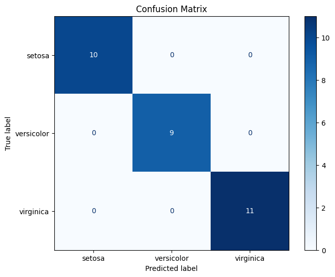
Confusion Matrix#
[5]:
# Get predictions
y_pred = clf.predict(X_test)

# Plot confusion matrix
cm = confusion_matrix(y_test, y_pred)
disp = ConfusionMatrixDisplay(confusion_matrix=cm, display_labels=iris.target_names)

fig, ax = plt.subplots(figsize=(8, 6))
disp.plot(ax=ax, cmap='Blues')
plt.title('Confusion Matrix')
plt.show()
Classification Report#
[6]:
print(classification_report(y_test, y_pred, target_names=iris.target_names))
              precision    recall  f1-score   support

      setosa       1.00      1.00      1.00        10
  versicolor       1.00      1.00      1.00         9
   virginica       1.00      1.00      1.00        11

    accuracy                           1.00        30
   macro avg       1.00      1.00      1.00        30
weighted avg       1.00      1.00      1.00        30
Summary#
In this tutorial, you learned how to:
✅ Train a multiclass classifier with boosters
✅ Interpret multiclass probability outputs
✅ Visualize confusion matrices
✅ Analyze per-class metrics
Next Steps#
Tutorial 05: Early Stopping — Prevent overfitting
Tutorial 07: Hyperparameter Tuning — Optimize performance