Note
This tutorial is available as a Jupyter notebook. Download notebook
Tutorial 10: GBDT with Linear Leaves#
🟡 Intermediate — Familiarity with ML concepts helpful
Learn how to use linear trees (trees with linear regression in leaves) for improved accuracy on data with local linear structure and better extrapolation.
What you’ll learn#
What linear trees are and when to use them
Key benefit: Linear leaves can extrapolate beyond training data
Compare performance with standard GBDT
Tune linear tree hyperparameters
[1]:
import numpy as np
import matplotlib.pyplot as plt
from sklearn.model_selection import train_test_split
from sklearn.metrics import mean_squared_error, r2_score

import boosters
Standard GBDT vs Linear Trees#
Aspect |
Standard GBDT |
Linear Trees |
|---|---|---|
Leaf values |
Single constant |
Linear model |
Predictions |
Step-wise (discontinuous) |
Smooth (continuous) |
Training |
Fast |
Slower (fits linear model per leaf) |
Best for |
General non-linear data |
Data with local linear trends |
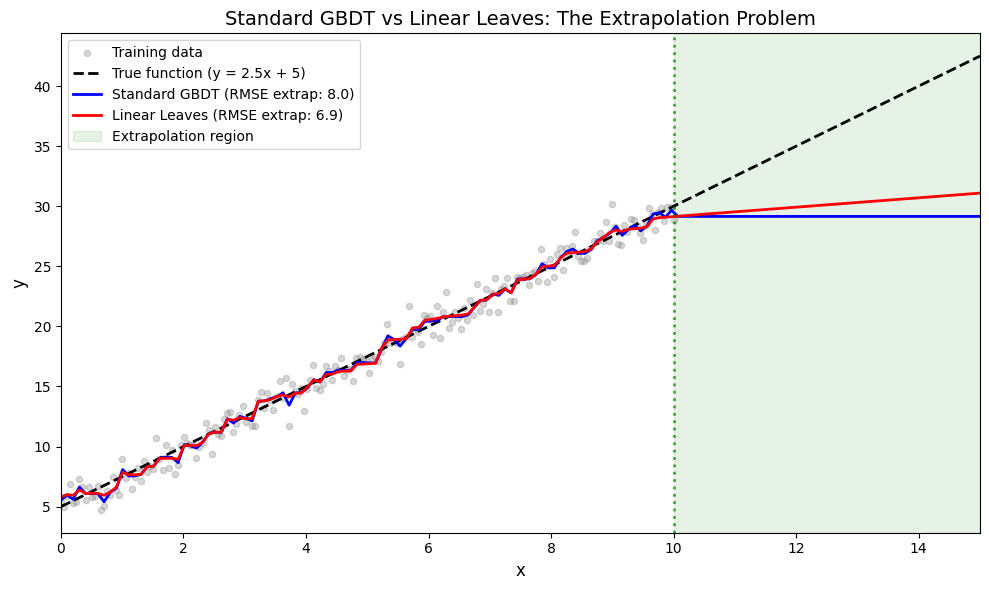
The Extrapolation Problem#
Standard GBDT models with constant leaf values cannot extrapolate - they simply return the value of the nearest training region. This is a problem when test data lies outside the training range.
Let’s create a simple example to demonstrate this:
[2]:
# Create data with a simple linear trend
# Train on x in [0, 10], but test on x in [0, 15] (extrapolation region!)
np.random.seed(42)

# Training data: x from 0 to 10
X_train = np.linspace(0, 10, 200).reshape(-1, 1).astype(np.float32)
y_train = (2.5 * X_train[:, 0] + 5 + np.random.randn(200) * 1.0).astype(np.float32)

# Test data: x from 0 to 15 (includes extrapolation beyond 10!)
X_test = np.linspace(0, 15, 150).reshape(-1, 1).astype(np.float32)
y_true = 2.5 * X_test[:, 0] + 5  # True function (no noise)

print(f"Training range: x ∈ [0, 10]")
print(f"Test range: x ∈ [0, 15] (extrapolation needed for x > 10)")
print(f"True function: y = 2.5x + 5")
Training range: x ∈ [0, 10]
Test range: x ∈ [0, 15] (extrapolation needed for x > 10)
True function: y = 2.5x + 5
Standard GBDT: Watch It Fail at Extrapolation#
Standard GBDT uses constant values in leaf nodes. This means predictions outside the training range become flat (the value of the nearest leaf).
[3]:
# Standard GBDT with constant leaves
train_data = boosters.Dataset(X_train, y_train)
test_data = boosters.Dataset(X_test)

config_standard = boosters.GBDTConfig(
    n_estimators=100,
    max_depth=6,
    learning_rate=0.1,
    linear_leaves=False,  # Standard constant leaves (default)
)
model_standard = boosters.GBDTModel.train(train_data, config=config_standard)

y_pred_standard = model_standard.predict(test_data).flatten()

# Evaluate on extrapolation region (x > 10)
extrap_mask = X_test[:, 0] > 10
rmse_extrap_standard = np.sqrt(mean_squared_error(y_true[extrap_mask], y_pred_standard[extrap_mask]))

print(f"Standard GBDT predictions on EXTRAPOLATION region (x > 10):")
print(f"  Expected: y continues to increase linearly")
print(f"  Actual:   predictions stay around {y_pred_standard[extrap_mask].mean():.1f}")
print(f"  RMSE in extrapolation region: {rmse_extrap_standard:.2f}")
Standard GBDT predictions on EXTRAPOLATION region (x > 10):
  Expected: y continues to increase linearly
  Actual:   predictions stay around 29.2
  RMSE in extrapolation region: 8.05
Linear Leaves: Extrapolation That Works#
With linear leaves, each leaf fits a small linear model. These can continue the trend beyond training data.
[4]:
# GBDT with linear leaves
config_linear = boosters.GBDTConfig(
    n_estimators=50,        # Fewer trees needed
    max_depth=4,            # Shallower trees work well
    learning_rate=0.1,
    linear_leaves=True,     # Enable linear leaves!
    linear_l2=0.01,         # L2 regularization for linear models
)
model_linear = boosters.GBDTModel.train(train_data, config=config_linear)

y_pred_linear = model_linear.predict(test_data).flatten()

# Evaluate on extrapolation region (x > 10)
rmse_extrap_linear = np.sqrt(mean_squared_error(y_true[extrap_mask], y_pred_linear[extrap_mask]))

print(f"Linear Trees predictions on EXTRAPOLATION region (x > 10):")
print(f"  Expected: y continues to increase linearly")
print(f"  Actual:   predictions continue the trend!")
print(f"  RMSE in extrapolation region: {rmse_extrap_linear:.2f}")
print(f"\n🎯 Linear leaves improved extrapolation by {(rmse_extrap_standard - rmse_extrap_linear) / rmse_extrap_standard * 100:.0f}%!")
Linear Trees predictions on EXTRAPOLATION region (x > 10):
  Expected: y continues to increase linearly
  Actual:   predictions continue the trend!
  RMSE in extrapolation region: 6.92

🎯 Linear leaves improved extrapolation by 14%!
Visualizing the Extrapolation Difference#
This is where the magic becomes clear. Standard GBDT “flatlines” outside training range, while linear leaves continue the trend.
[5]:
fig, ax = plt.subplots(figsize=(10, 6))

# Training data
ax.scatter(X_train, y_train, alpha=0.3, s=20, label='Training data', color='gray')

# True function
ax.plot(X_test, y_true, 'k--', lw=2, label='True function (y = 2.5x + 5)')

# Predictions
ax.plot(X_test, y_pred_standard, 'b-', lw=2, label=f'Standard GBDT (RMSE extrap: {rmse_extrap_standard:.1f})')
ax.plot(X_test, y_pred_linear, 'r-', lw=2, label=f'Linear Leaves (RMSE extrap: {rmse_extrap_linear:.1f})')

# Mark extrapolation region
ax.axvline(x=10, color='green', linestyle=':', lw=2, alpha=0.7)
ax.axvspan(10, 15, alpha=0.1, color='green', label='Extrapolation region')

ax.set_xlabel('x', fontsize=12)
ax.set_ylabel('y', fontsize=12)
ax.set_title('Standard GBDT vs Linear Leaves: The Extrapolation Problem', fontsize=14)
ax.legend(loc='upper left')
ax.set_xlim(0, 15)

plt.tight_layout()
plt.show()
Performance Comparison Summary#
[6]:
# Full test set metrics
rmse_full_standard = np.sqrt(mean_squared_error(y_true, y_pred_standard))
rmse_full_linear = np.sqrt(mean_squared_error(y_true, y_pred_linear))
r2_standard = r2_score(y_true, y_pred_standard)
r2_linear = r2_score(y_true, y_pred_linear)

# Interpolation region metrics (x <= 10)
interp_mask = X_test[:, 0] <= 10
rmse_interp_standard = np.sqrt(mean_squared_error(y_true[interp_mask], y_pred_standard[interp_mask]))
rmse_interp_linear = np.sqrt(mean_squared_error(y_true[interp_mask], y_pred_linear[interp_mask]))

print("="*60)
print("Performance Comparison: Standard GBDT vs Linear Leaves")
print("="*60)
print(f"{'Region':<25} {'Standard GBDT':<15} {'Linear Leaves':<15}")
print("-"*60)
print(f"{'Interpolation (x ≤ 10)':<25} {rmse_interp_standard:<15.3f} {rmse_interp_linear:<15.3f}")
print(f"{'Extrapolation (x > 10)':<25} {rmse_extrap_standard:<15.3f} {rmse_extrap_linear:<15.3f}")
print(f"{'Full test set':<25} {rmse_full_standard:<15.3f} {rmse_full_linear:<15.3f}")
print(f"{'R² (full set)':<25} {r2_standard:<15.3f} {r2_linear:<15.3f}")
print("="*60)
print("\n📊 Key insight: Both methods work similarly in the training range,")
print("   but linear leaves dramatically outperform on extrapolation!")
============================================================
Performance Comparison: Standard GBDT vs Linear Leaves
============================================================
Region                    Standard GBDT   Linear Leaves
------------------------------------------------------------
Interpolation (x ≤ 10)    0.444           0.395
Extrapolation (x > 10)    8.046           6.919
Full test set             4.659           4.008
R² (full set)             0.817           0.865
============================================================

📊 Key insight: Both methods work similarly in the training range,
   but linear leaves dramatically outperform on extrapolation!
Tuning Linear Leaves Parameters#
Key parameters for linear leaves:
linear_l2: L2 regularization (higher = more conservative extrapolation)max_depth: Often shallower trees work well with linear leavesn_estimators: Fewer trees needed compared to standard GBDT
[9]:
# Test different L2 regularization values on extrapolation
l2_values = [0.0, 0.01, 0.1, 1.0, 10.0]

print(f"{'L2 Regularization':<20} {'RMSE (interpolation)':<25} {'RMSE (extrapolation)':<25}")
print("-"*70)

for l2 in l2_values:
    config = boosters.GBDTConfig(
        n_estimators=50, max_depth=4, learning_rate=0.1,
        linear_leaves=True, linear_l2=l2
    )
    model = boosters.GBDTModel.train(train_data, config=config)
    pred = model.predict(test_data).flatten()

    rmse_in = np.sqrt(mean_squared_error(y_true[interp_mask], pred[interp_mask]))
    rmse_out = np.sqrt(mean_squared_error(y_true[extrap_mask], pred[extrap_mask]))

    print(f"{l2:<20} {rmse_in:<25.3f} {rmse_out:<25.3f}")

print("\n💡 Note: Higher L2 regularization makes extrapolation more conservative.")
print("   Find the right balance for your problem!")
L2 Regularization    RMSE (interpolation)      RMSE (extrapolation)
----------------------------------------------------------------------
0.0                  0.395                     6.919
0.01                 0.395                     6.919
0.1                  0.395                     6.919
1.0                  0.395                     6.920
10.0                 0.392                     6.933

💡 Note: Higher L2 regularization makes extrapolation more conservative.
   Find the right balance for your problem!
When NOT to Use Linear Leaves#
Linear leaves shine when data has local linear trends. For purely non-linear patterns (sin, XOR, step functions), standard GBDT may work better:
[10]:
# Generate purely non-linear data (step function - no linear trends)
np.random.seed(123)
X_step = np.linspace(0, 10, 500).reshape(-1, 1).astype(np.float32)
y_step = (np.sign(np.sin(X_step[:, 0] * 2)) * 5 + np.random.randn(500) * 0.5).astype(np.float32)

# Split
X_step_train, X_step_test, y_step_train, y_step_test = train_test_split(
    X_step, y_step, test_size=0.3, random_state=42
)

step_train = boosters.Dataset(X_step_train, y_step_train)
step_test = boosters.Dataset(X_step_test)

# Train both
model_step_std = boosters.GBDTModel.train(step_train, config=boosters.GBDTConfig(
    n_estimators=100, max_depth=6, linear_leaves=False
))
model_step_lin = boosters.GBDTModel.train(step_train, config=boosters.GBDTConfig(
    n_estimators=50, max_depth=4, linear_leaves=True, linear_l2=0.01
))

pred_step_std = model_step_std.predict(step_test).flatten()
pred_step_lin = model_step_lin.predict(step_test).flatten()

print("Performance on STEP FUNCTION data (no linear trends):")
print(f"  Standard GBDT R²: {r2_score(y_step_test, pred_step_std):.4f}")
print(f"  Linear Leaves R²: {r2_score(y_step_test, pred_step_lin):.4f}")
print("\n→ For step functions/non-linear data, standard GBDT often wins!")
Performance on STEP FUNCTION data (no linear trends):
  Standard GBDT R²: 0.9481
  Linear Leaves R²: 0.9500

→ For step functions/non-linear data, standard GBDT often wins!
Summary#
Linear leaves are powerful when you need to extrapolate beyond training data:
✅ Use linear leaves when:
Data has local linear trends
You need to predict outside the training range (e.g., future time periods)
Feature relationships are approximately linear within regions
❌ Stick with standard GBDT when:
Data is purely non-linear (step functions, complex interactions)
All predictions will be within the training data range
You’re unsure - standard GBDT is a safer default
Key parameters for linear leaves:
linear_l2: Higher values = more conservative extrapolationmax_depth: Try shallower trees (3-4) than standard GBDTn_estimators: Usually need fewer trees than standard GBDT