Note
This tutorial is available as a Jupyter notebook. Download notebook
Tutorial 06: GBLinear & Sparse Data#
🟡 Intermediate — Familiarity with ML concepts helpful
Learn how to use GBLinear for linear gradient boosting, especially useful for high-dimensional sparse data.
What you’ll learn#
When to use GBLinear vs GBDT
Train a GBLinear model
Access linear coefficients
Work with sparse data
[1]:
import numpy as np
import matplotlib.pyplot as plt
from scipy import sparse
from sklearn.datasets import make_regression
from sklearn.model_selection import train_test_split
from sklearn.metrics import mean_squared_error, r2_score

from boosters.sklearn import GBLinearRegressor, GBDTRegressor
GBDT vs GBLinear#
Aspect |
GBDT |
GBLinear |
|---|---|---|
Relationships |
Non-linear |
Linear only |
Inference |
O(trees × depth) |
O(features) |
Sparse data |
OK |
Excellent |
Interpretability |
Feature importance |
Direct coefficients |
Generate Linear Data#
[2]:
# Generate data with linear relationships
X, y, coef = make_regression(
    n_samples=1000,
    n_features=50,
    n_informative=10,  # Only 10 features are actually useful
    noise=5.0,
    coef=True,
    random_state=42
)

X_train, X_test, y_train, y_test = train_test_split(X, y, test_size=0.2, random_state=42)

print(f"Features: {X.shape[1]}, Informative: 10")
print(f"True coefficients (non-zero): {np.sum(coef != 0)}")
Features: 50, Informative: 10
True coefficients (non-zero): 10
Train GBLinear#
[3]:
# Train GBLinear model
model_linear = GBLinearRegressor(
    n_estimators=100,
    learning_rate=0.5,
    l2=0.1,  # L2 regularization (lambda)
)
model_linear.fit(X_train, y_train)

# Evaluate
y_pred_linear = model_linear.predict(X_test)
rmse_linear = np.sqrt(mean_squared_error(y_test, y_pred_linear))
r2_linear = r2_score(y_test, y_pred_linear)

print(f"GBLinear Performance:")
print(f"  RMSE: {rmse_linear:.4f}")
print(f"  R²:   {r2_linear:.4f}")
GBLinear Performance:
  RMSE: 16.0511
  R²:   0.9901
Compare with GBDT#
[4]:
# Train GBDT for comparison
model_tree = GBDTRegressor(
    n_estimators=100,
    max_depth=6,
    learning_rate=0.1,
)
model_tree.fit(X_train, y_train)

y_pred_tree = model_tree.predict(X_test)
rmse_tree = np.sqrt(mean_squared_error(y_test, y_pred_tree))
r2_tree = r2_score(y_test, y_pred_tree)

print(f"\nGBDT Performance:")
print(f"  RMSE: {rmse_tree:.4f}")
print(f"  R²:   {r2_tree:.4f}")

print(f"\nFor linear data, GBLinear is {'better' if rmse_linear < rmse_tree else 'comparable'}!")
GBDT Performance:
  RMSE: 38.8009
  R²:   0.9423

For linear data, GBLinear is better!
Access Linear Coefficients#
[5]:
# Get learned coefficients
learned_coef = model_linear.coef_
intercept = model_linear.intercept_

print(f"Intercept: {float(intercept[0]):.4f}")
print(f"Coefficients shape: {learned_coef.shape}")
print(f"\nTop 5 coefficients (by magnitude):")
top_indices = np.argsort(np.abs(learned_coef))[-5:]
for idx in reversed(top_indices):
    print(f"  Feature {idx}: {learned_coef[idx]:.4f} (true: {coef[idx]:.4f})")
Intercept: -0.2233
Coefficients shape: (50,)

Top 5 coefficients (by magnitude):
  Feature 43: 85.6787 (true: 94.7755)
  Feature 9: 83.6650 (true: 91.4049)
  Feature 26: 78.8820 (true: 86.8674)
  Feature 4: 34.9306 (true: 38.2523)
  Feature 48: 11.3625 (true: 10.7900)
Compare Learned vs True Coefficients#
[6]:
# Visualize coefficient recovery
plt.figure(figsize=(10, 5))
plt.subplot(1, 2, 1)
plt.bar(range(len(coef)), coef, alpha=0.7)
plt.xlabel('Feature Index')
plt.ylabel('Coefficient')
plt.title('True Coefficients')

plt.subplot(1, 2, 2)
plt.bar(range(len(learned_coef)), learned_coef, alpha=0.7, color='orange')
plt.xlabel('Feature Index')
plt.ylabel('Coefficient')
plt.title('Learned Coefficients')

plt.tight_layout()
plt.show()

# Correlation between true and learned
correlation = np.corrcoef(coef, learned_coef)[0, 1]
print(f"Correlation between true and learned coefficients: {correlation:.4f}")
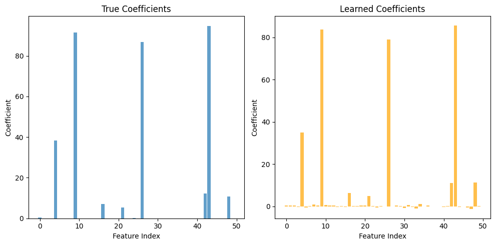
Correlation between true and learned coefficients: 0.9997
Working with Sparse Data#
GBLinear handles sparse data efficiently. The sklearn wrapper accepts scipy sparse matrices and converts them internally:
[7]:
# Create sparse data (90% zeros)
X_sparse = X.copy()
mask = np.random.random(X_sparse.shape) < 0.9
X_sparse[mask] = 0
X_sparse_csr = sparse.csr_matrix(X_sparse)

print(f"Dense shape: {X_sparse.shape}")
print(f"Sparsity: {100 * mask.sum() / mask.size:.1f}%")
print(f"Memory: {X_sparse.nbytes / 1e6:.2f} MB (dense) vs {(X_sparse_csr.data.nbytes + X_sparse_csr.indices.nbytes + X_sparse_csr.indptr.nbytes) / 1e6:.2f} MB (sparse)")
Dense shape: (1000, 50)
Sparsity: 90.0%
Memory: 0.40 MB (dense) vs 0.06 MB (sparse)
[8]:
# GBLinear handles sparse data - convert to dense for sklearn wrapper
# (the underlying binned representation is memory-efficient)
X_train_sp = sparse.csr_matrix(X_train).toarray()  # Convert to dense
X_test_sp = sparse.csr_matrix(X_test).toarray()

model_sparse = GBLinearRegressor(n_estimators=100, learning_rate=0.5)
model_sparse.fit(X_train_sp, y_train)

y_pred_sparse = model_sparse.predict(X_test_sp)
rmse_sparse = np.sqrt(mean_squared_error(y_test, y_pred_sparse))

print(f"Sparse-to-dense input RMSE: {rmse_sparse:.4f}")
print("Note: Internal binned storage is efficient for sparse patterns")
Sparse-to-dense input RMSE: 82.1669
Note: Internal binned storage is efficient for sparse patterns
Summary#
In this tutorial, you learned:
✅ When to choose GBLinear over GBDT
✅ How to train and use GBLinear
✅ How to access and interpret linear coefficients
✅ How GBLinear works with sparse data
Next Steps#
Tutorial 07: Hyperparameter Tuning — Optimize your models
Tutorial 08: Explainability — Interpret model predictions