Note
This tutorial is available as a Jupyter notebook. Download notebook
Tutorial 08: Explainability#
🟡 Intermediate — Familiarity with ML concepts helpful
Learn how to interpret boosted model predictions using feature importance and SHAP values.
What you’ll learn#
Built-in feature importance (split-based)
SHAP values for local explanations
Visualizing feature contributions
Interpreting GBLinear coefficients
[1]:
import numpy as np
import matplotlib.pyplot as plt
from sklearn.datasets import fetch_california_housing
from sklearn.model_selection import train_test_split

import boosters
from boosters.sklearn import GBDTRegressor, GBLinearRegressor
Load California Housing Dataset#
We’ll use the California housing dataset which has meaningful, interpretable feature names:
[2]:
# Load California housing - predicting median house value
data = fetch_california_housing()
X, y = data.data, data.target
feature_names = data.feature_names

X_train, X_test, y_train, y_test = train_test_split(X, y, test_size=0.2, random_state=42)

print("California Housing Dataset")
print(f"Samples: {len(X)}, Features: {len(feature_names)}")
print(f"\nFeature names:")
for i, name in enumerate(feature_names):
    print(f"  {i}: {name}")
California Housing Dataset
Samples: 20640, Features: 8

Feature names:
  0: MedInc
  1: HouseAge
  2: AveRooms
  3: AveBedrms
  4: Population
  5: AveOccup
  6: Latitude
  7: Longitude
Train Model#
[3]:
# Train GBDT regressor
model = GBDTRegressor(n_estimators=100, max_depth=6, learning_rate=0.1)
model.fit(X_train, y_train)

print(f"R² Score: {model.score(X_test, y_test):.4f}")
R² Score: 0.8247
Built-in Feature Importance#
GBDT models track feature importance based on split gain:
[4]:
# Get feature importance
importance = model.feature_importances_

# Sort by importance
indices = np.argsort(importance)[::-1]

# Plot
plt.figure(figsize=(10, 5))
plt.barh(range(len(importance)), importance[indices][::-1])
plt.yticks(range(len(importance)), [feature_names[i] for i in indices][::-1])
plt.xlabel('Importance (Gain)')
plt.title('Feature Importance - California Housing')
plt.tight_layout()
plt.show()

print("\nTop features for predicting house value:")
for i in indices[:5]:
    print(f"  {feature_names[i]}: {importance[i]:.4f}")
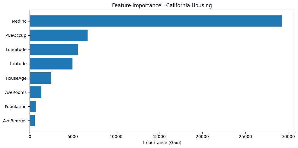
Top features for predicting house value:
  MedInc: 29231.8770
  AveOccup: 6699.3140
  Longitude: 5577.1704
  Latitude: 4971.0332
  HouseAge: 2475.5881
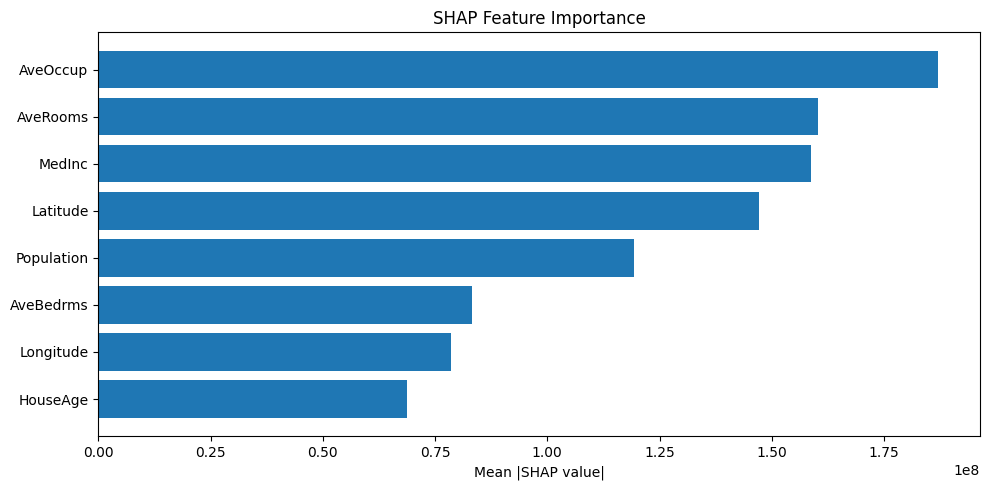
SHAP Values#
SHAP (SHapley Additive exPlanations) values show how each feature contributes to individual predictions:
[5]:
# Calculate SHAP values for first 100 test samples
# Access the underlying model via model_ and wrap data in Dataset
shap_values = model.model_.shap_values(boosters.Dataset(X_test[:100]))

print(f"SHAP values shape: {shap_values.shape}")
print(f"  (samples, features + 1 bias, outputs)")

# Mean absolute SHAP value per feature (global importance)
# Shape is (samples, features+1, outputs) - take first output, exclude bias
mean_shap = np.abs(shap_values[:, :-1, 0]).mean(axis=0)
shap_indices = np.argsort(mean_shap)[::-1]

plt.figure(figsize=(10, 5))
plt.barh(range(len(mean_shap)), mean_shap[shap_indices][::-1])
plt.yticks(range(len(mean_shap)), [feature_names[i] for i in shap_indices][::-1])
plt.xlabel('Mean |SHAP value|')
plt.title('SHAP Feature Importance')
plt.tight_layout()
plt.show()
SHAP values shape: (100, 9, 1)
  (samples, features + 1 bias, outputs)
Explain a Single Prediction#
Let’s explain why the model predicted a specific house value:
[6]:
# Pick a sample to explain
sample_idx = 0
sample = X_test[sample_idx]
prediction = model.predict(sample.reshape(1, -1))[0]
actual = y_test[sample_idx]

print(f"Prediction: ${prediction * 100000:.0f}")
print(f"Actual:     ${actual * 100000:.0f}")
print(f"\nFeature contributions (SHAP values):")

# Get SHAP values for this sample (first output, exclude bias)
sample_shap = shap_values[sample_idx, :-1, 0]
bias = shap_values[sample_idx, -1, 0]

# Waterfall-style breakdown
contributions = list(zip(feature_names, sample_shap, sample))
contributions.sort(key=lambda x: abs(x[1]), reverse=True)

print(f"\nBase value (bias): {bias:.3f}")
for name, shap_val, feat_val in contributions:
    direction = "↑" if shap_val > 0 else "↓"
    print(f"  {name}={feat_val:.2f}: {shap_val:+.3f} {direction}")
Prediction: $56112
Actual:     $47700

Feature contributions (SHAP values):

Base value (bias): 2.072
  MedInc=1.68: -238035952.000 ↓
  Longitude=-119.01: -60131828.000 ↓
  Latitude=36.06: -57731232.000 ↓
  AveOccup=3.88: +46847604.000 ↑
  AveBedrms=1.02: +41947896.000 ↑
  Population=1392.00: +33873256.000 ↑
  AveRooms=4.19: -22673940.000 ↓
  HouseAge=25.00: +14655487.000 ↑
GBLinear: Direct Coefficient Interpretation#
Linear models have directly interpretable coefficients:
[7]:
# Train GBLinear for comparison
linear_model = GBLinearRegressor(n_estimators=100, learning_rate=0.3)
linear_model.fit(X_train, y_train)

print(f"GBLinear R² Score: {linear_model.score(X_test, y_test):.4f}")
GBLinear R² Score: 0.4786
[8]:
# Get coefficients - directly interpretable!
coef = linear_model.coef_

# Sort by absolute value
coef_indices = np.argsort(np.abs(coef))[::-1]

# Plot
plt.figure(figsize=(10, 5))
colors = ['green' if c > 0 else 'red' for c in coef[coef_indices][::-1]]
plt.barh(range(len(coef)), coef[coef_indices][::-1], color=colors)
plt.yticks(range(len(coef)), [feature_names[i] for i in coef_indices][::-1])
plt.xlabel('Coefficient')
plt.title('GBLinear Coefficients - California Housing')
plt.axvline(x=0, color='black', linestyle='-', linewidth=0.5)
plt.tight_layout()
plt.show()

print("Interpretation:")
print("  Green = higher value → higher house price")
print("  Red = higher value → lower house price")
print(f"\nIntercept: {float(linear_model.intercept_[0]):.4f}")
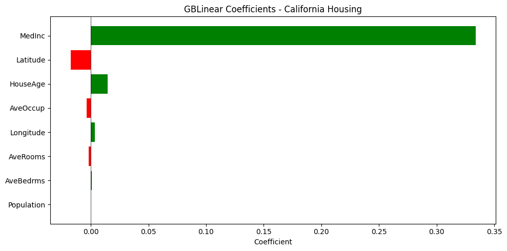
Interpretation:
  Green = higher value → higher house price
  Red = higher value → lower house price

Intercept: 1.4166
Summary#
In this tutorial, you learned:
✅ Built-in feature importance from split gain
✅ SHAP values for local explanations of individual predictions
✅ How to interpret which features drive predictions
✅ Direct coefficient interpretation with GBLinear
Key insights from California Housing:
MedInc(median income) is the strongest predictor of house valueLocation features (
Latitude,Longitude) capture geographic price variationAveOccup(average occupancy) andHouseAgealso contribute
Next Steps#
Tutorial 09: Model Serialization — Save and load models
User Guide: Explainability — Full documentation