Note
This tutorial is available as a Jupyter notebook. Download notebook
Tutorial 11: Sample Weighting#
🟡 Intermediate — Familiarity with ML concepts helpful
Learn how to use sample weights to handle class imbalance, emphasize recent data, and downweight outliers.
What you’ll learn#
Handle class imbalance with balanced sample weights
Use temporal weighting for concept drift
Downweight outliers and noisy samples
Integrate sample weights with both sklearn and core APIs
[1]:
import numpy as np
from sklearn.datasets import make_classification
from sklearn.metrics import classification_report
from sklearn.model_selection import train_test_split
from sklearn.utils.class_weight import compute_sample_weight

import boosters
from boosters.sklearn import GBDTClassifier, GBDTRegressor
Why Sample Weights?#
Sample weights allow you to control how much each training example contributes to the model:
Class imbalance: Give minority class samples higher weights
Temporal importance: Weight recent data more heavily for concept drift
Data quality: Downweight known outliers or noisy samples
Business logic: Emphasize high-value customers or critical cases
1. Handling Class Imbalance#
When classes are imbalanced, the model tends to favor the majority class. Sample weights can correct this by giving minority samples more importance.
[2]:
# Create imbalanced dataset (95% class 0, 5% class 1)
rng = np.random.default_rng(42)
n_samples = 1000
n_minority = 50

X = rng.standard_normal((n_samples, 5)).astype(np.float32)

# Create imbalanced labels
y = np.zeros(n_samples, dtype=np.float32)
y[:n_minority] = 1.0

# Shuffle
perm = rng.permutation(n_samples)
X, y = X[perm], y[perm]

X_train, X_test, y_train, y_test = train_test_split(
    X, y, test_size=0.2, random_state=42, stratify=y
)

print(f"Class distribution in training: {np.bincount(y_train.astype(int))}")
print(f"Class distribution in test:     {np.bincount(y_test.astype(int))}")
Class distribution in training: [760  40]
Class distribution in test:     [190  10]
Without Sample Weights#
The model will likely predict only the majority class:
[3]:
clf_no_weights = GBDTClassifier(n_estimators=50, verbose=0)
clf_no_weights.fit(X_train, y_train)
pred_no_weights = clf_no_weights.predict(X_test)

print("Classification Report (no weights):")
print(classification_report(y_test, pred_no_weights, zero_division=0))
Classification Report (no weights):
              precision    recall  f1-score   support

         0.0       0.95      1.00      0.97       190
         1.0       0.00      0.00      0.00        10

    accuracy                           0.95       200
   macro avg       0.47      0.50      0.49       200
weighted avg       0.90      0.95      0.93       200
With Balanced Sample Weights#
sklearn’s compute_sample_weight calculates weights inversely proportional to class frequency:
[4]:
# Compute balanced weights
weights = compute_sample_weight("balanced", y_train)

print(f"Weight for class 0 samples: {weights[y_train == 0][0]:.3f}")
print(f"Weight for class 1 samples: {weights[y_train == 1][0]:.3f}")
print(f"Ratio: {weights[y_train == 1][0] / weights[y_train == 0][0]:.1f}x")
Weight for class 0 samples: 0.526
Weight for class 1 samples: 10.000
Ratio: 19.0x
[5]:
clf_weighted = GBDTClassifier(n_estimators=50, verbose=0)
clf_weighted.fit(X_train, y_train, sample_weight=weights)
pred_weighted = clf_weighted.predict(X_test)

print("Classification Report (with balanced weights):")
print(classification_report(y_test, pred_weighted, zero_division=0))
Classification Report (with balanced weights):
              precision    recall  f1-score   support

         0.0       0.95      0.93      0.94       190
         1.0       0.00      0.00      0.00        10

    accuracy                           0.89       200
   macro avg       0.47      0.47      0.47       200
weighted avg       0.90      0.89      0.89       200
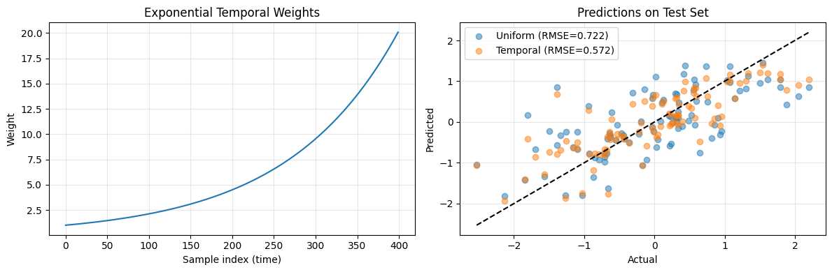
2. Temporal Weighting for Concept Drift#
When data distribution changes over time (concept drift), you may want to emphasize recent observations. This is common in:
Financial markets
User behavior prediction
Fraud detection
[6]:
# Simulate temporal data with concept drift
rng = np.random.default_rng(42)
n_samples = 500

X = rng.standard_normal((n_samples, 3)).astype(np.float32)

# Target relationship changes over time:
# Early: y depends mostly on X[:, 0]
# Late: y depends mostly on X[:, 1]
time_factor = np.linspace(0, 1, n_samples)
y = ((1 - time_factor) * X[:, 0] + time_factor * X[:, 1]).astype(np.float32)
y += rng.standard_normal(n_samples).astype(np.float32) * 0.1

# Split chronologically (not randomly!)
train_size = 400
X_train, X_test = X[:train_size], X[train_size:]
y_train, y_test = y[:train_size], y[train_size:]

print(f"Training on first {train_size} samples")
print(f"Testing on last {n_samples - train_size} samples (most recent)")
Training on first 400 samples
Testing on last 100 samples (most recent)
[7]:
# Uniform weights baseline
reg_uniform = GBDTRegressor(n_estimators=50, verbose=0)
reg_uniform.fit(X_train, y_train)
pred_uniform = reg_uniform.predict(X_test)
rmse_uniform = np.sqrt(np.mean((pred_uniform - y_test) ** 2))

# Exponential decay weights - recent samples have higher weight
decay_rate = 3.0  # Higher = more emphasis on recent data
temporal_weights = np.exp(decay_rate * np.linspace(0, 1, train_size)).astype(np.float32)

reg_weighted = GBDTRegressor(n_estimators=50, verbose=0)
reg_weighted.fit(X_train, y_train, sample_weight=temporal_weights)
pred_weighted = reg_weighted.predict(X_test)
rmse_weighted = np.sqrt(np.mean((pred_weighted - y_test) ** 2))

print(f"RMSE with uniform weights:   {rmse_uniform:.4f}")
print(f"RMSE with temporal weights:  {rmse_weighted:.4f}")
print(f"Improvement: {(rmse_uniform - rmse_weighted) / rmse_uniform * 100:.1f}%")
RMSE with uniform weights:   0.7219
RMSE with temporal weights:  0.5716
Improvement: 20.8%
[8]:
import matplotlib.pyplot as plt

fig, (ax1, ax2) = plt.subplots(1, 2, figsize=(12, 4))

# Plot weight distribution
ax1.plot(temporal_weights)
ax1.set_xlabel("Sample index (time)")
ax1.set_ylabel("Weight")
ax1.set_title("Exponential Temporal Weights")
ax1.grid(True, alpha=0.3)

# Plot predictions vs actual
ax2.scatter(y_test, pred_uniform, alpha=0.5, label=f"Uniform (RMSE={rmse_uniform:.3f})")
ax2.scatter(y_test, pred_weighted, alpha=0.5, label=f"Temporal (RMSE={rmse_weighted:.3f})")
ax2.plot([y_test.min(), y_test.max()], [y_test.min(), y_test.max()], "k--")
ax2.set_xlabel("Actual")
ax2.set_ylabel("Predicted")
ax2.set_title("Predictions on Test Set")
ax2.legend()
ax2.grid(True, alpha=0.3)

plt.tight_layout()
plt.show()
3. Downweighting Outliers#
If you know certain samples are outliers or noisy, you can reduce their influence:
[9]:
rng = np.random.default_rng(42)
X = rng.standard_normal((200, 4)).astype(np.float32)
y = (X[:, 0] + X[:, 1] * 0.5 + rng.standard_normal(200) * 0.1).astype(np.float32)

# Inject some outliers
outlier_idx = [10, 50, 100, 150]
y[outlier_idx] = y[outlier_idx] + 10.0  # Shift by 10 standard deviations

# Create weights - downweight outliers
weights = np.ones(200, dtype=np.float32)
weights[outlier_idx] = 0.01  # Very low weight for known outliers

print(f"Number of outliers: {len(outlier_idx)}")
print(f"Outlier weight: {weights[outlier_idx[0]]}")
Number of outliers: 4
Outlier weight: 0.009999999776482582
[10]:
# Without outlier handling
reg_no_handling = GBDTRegressor(n_estimators=50, verbose=0)
reg_no_handling.fit(X, y)
pred_no_handling = reg_no_handling.predict(X)

# With outlier downweighting
reg_downweight = GBDTRegressor(n_estimators=50, verbose=0)
reg_downweight.fit(X, y, sample_weight=weights)
pred_downweight = reg_downweight.predict(X)

# Calculate RMSE on non-outlier samples only
mask = ~np.isin(np.arange(len(y)), outlier_idx)
rmse_no = np.sqrt(np.mean((pred_no_handling[mask] - y[mask]) ** 2))
rmse_dw = np.sqrt(np.mean((pred_downweight[mask] - y[mask]) ** 2))

print(f"RMSE on clean samples (no handling):    {rmse_no:.4f}")
print(f"RMSE on clean samples (with weights):   {rmse_dw:.4f}")
RMSE on clean samples (no handling):    0.2987
RMSE on clean samples (with weights):   0.1037
4. Core API with Sample Weights#
You can also use sample weights directly with the core Dataset and GBDTModel API:
[11]:
from boosters import Dataset, GBDTConfig, GBDTModel, Objective

rng = np.random.default_rng(42)
X = rng.standard_normal((200, 4)).astype(np.float32)
y = (X[:, 0] + X[:, 1] * 0.5 + rng.standard_normal(200) * 0.1).astype(np.float32)

# Create custom weights
weights = np.ones(200, dtype=np.float32)
weights[np.abs(y) > 2] = 0.1  # Downweight extreme values

print(f"Samples with reduced weight: {np.sum(weights < 1)}")
Samples with reduced weight: 17
[12]:
# Create dataset WITH weights
train_data = Dataset(
    X, y,
    weights=weights,
    feature_names=["feat_a", "feat_b", "feat_c", "feat_d"]
)

config = GBDTConfig(
    n_estimators=50,
    max_depth=4,
    learning_rate=0.1,
    objective=Objective.squared(),
)

model = GBDTModel.train(train_data, config=config)
predictions = model.predict(Dataset(X))

rmse = np.sqrt(np.mean((predictions.flatten() - y) ** 2))
print(f"Training RMSE: {rmse:.4f}")
print(f"Feature names stored in model: {model.feature_names}")
Training RMSE: 0.2142
Feature names stored in model: ['feat_a', 'feat_b', 'feat_c', 'feat_d']
Summary#
Sample weights are a powerful tool for:
Use Case |
Weight Strategy |
|---|---|
Class imbalance |
Inverse class frequency ( |
Concept drift |
Exponential decay (recent → higher weight) |
Known outliers |
Low fixed weight (e.g., 0.01) |
Business importance |
Custom weights per sample |
Key Points#
sklearn API: Pass
sample_weightto.fit()Core API: Pass
weightstoDataset()Weights are relative — they don’t need to sum to 1
Use
compute_sample_weight("balanced")for quick class balancingFor temporal weighting, use exponential decay:
exp(rate * normalized_time)
Next Steps#
Tutorial 07: Hyperparameter Tuning — Optimize model performance
Tutorial 08: Explainability — Understand model predictions
User Guide: Recipes — Common patterns and solutions